Demand forecasting estimates how much customers may buy in a future period using information available today. A planner uses that estimate to prepare purchasing, production, or replenishment decisions. A forecast is not a promise—and recorded sales are not always the same as demand when products are out of stock.
In this illustrated example, I compare two simple forecasting methods on one product from a public retail dataset. You can explore the weekly calculations yourself before looking at the overall result.
What is the planning question?
Imagine preparing next week’s stock for a single online-retail product. You know its previous weekly sales, but not next week’s sales. Would you repeat last week, average the last four weeks, or use an exponentially smoothed estimate? A useful method should be understandable, reproducible, and tested against weeks it has not yet seen.
This example uses product code 22423 in the UCI Online Retail dataset. I treat positive transaction quantities as observed sales. The file does not tell us whether a stockout prevented additional sales, so these numbers are not a complete measure of customer demand.
How do the methods work?
Four-week moving average
A moving average gives each of the four latest completed weeks equal weight. For the week starting 10 October 2011, the previous four sales totals were 219, 147, 149, and 409 units. Their mean is (219 + 147 + 149 + 409) ÷ 4 = 231 units. This becomes the one-week-ahead forecast. When a new week ends, the oldest value leaves the four-week window and the newly observed value enters it.
Simple exponential smoothing
Exponential smoothing updates a running level rather than keeping an equally weighted four-week window. Here, the updated level is 0.30 × this week’s actual sales + 0.70 × the previous level; the updated level forecasts the next week. Older observations still influence that level, but their influence decreases over time. I fixed α at 0.30 as an illustrative setting, initialized the level with the first observed week, and did not tune α on the test weeks.
For a fair reference point, I also use a naïve baseline: predict that next week will equal the most recent completed week. A method should earn its complexity by beating a simple alternative.
Explore the eight test weeks
Select a week to see the four earlier sales totals used by the moving average, then compare its forecast with exponential smoothing and the actual sales.
Week starting 10 Oct 2011 · Product 22423 · units
(219 + 147 + 149 + 409) ÷ 4 = 231.0 units
In this week, the four-week average missed actual sales by 17.0 units.
Illustrative product from Chen (2015), UCI Online Retail. Forecasts use only earlier weeks; actual sales are revealed here for evaluation, not used to predict that week. The smoothing forecast uses α = 0.30 and all prior observations.
Try switching weeks above. The selected date is the week being predicted. The four earlier bars show the moving-average inputs; the comparison bars show predictions and the later-observed actual. No method uses the selected week’s actual before making its forecast.
What happened in the eight held-out weeks?
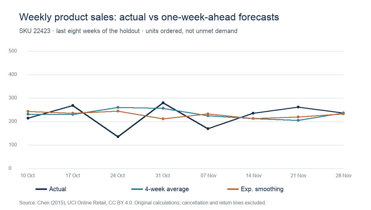
For product code 22423, the four-week moving average had the lowest mean absolute error (MAE): 42.1 units per week across the eight held-out weeks. Simple exponential smoothing was close at 46.2 units; predicting the previous week’s sales was much less accurate at 94.1 units. This is one product and one short test window, not evidence that moving averages are best for every SKU.
| One-week-ahead method | MAE, units/week | WAPE | Mean error, forecast minus actual |
|---|---|---|---|
| Four-week moving average | 42.1 | 18.7% | +7.2 units |
| Simple exponential smoothing (α = 0.30) | 46.2 | 20.6% | +4.1 units |
| Last-week naïve baseline | 94.1 | 41.9% | +21.6 units |
How I prepared the sales series
- I selected product code 22423 as an illustrative, frequently sold SKU. This choice is exploratory, not a random or pre-registered sample.
- I used 52 complete Monday–Sunday weeks, from 6 December 2010 through 4 December 2011. I excluded cancellation invoices, returned or non-positive quantities, and non-positive prices. The resulting series has 1,935 transaction lines and 12,881 positive units.
- I summed quantity by week. One week with no retained transaction was entered as zero recorded sales; that does not prove customer demand was zero.
- I held out the final eight weeks, 10 October–4 December 2011. The chart labels weeks by their Monday start dates; the last start date is 28 November.
How the forecasts were tested
Each forecast predicts one week ahead using only values known before that week. The naïve forecast repeats the previous week’s actual units. The moving average takes the mean of the four preceding weeks. Exponential smoothing uses levelt = 0.30 × actualt + 0.70 × levelt−1, initialized with the first observed week. The 0.30 weight is an illustrative fixed choice; it was not optimized on the holdout. After each test week, the methods receive that week’s actual before predicting the next one. This is rolling one-step evaluation, not an eight-week forecast issued at one time.
MAE is the average absolute difference between forecast and actual units. WAPE is the sum of absolute errors divided by the sum of actual units across the eight weeks. The denominator is positive here, so WAPE is defined. Mean signed error shows over- or underforecasting; a positive value means overforecasting.
What a planner can—and cannot—conclude
The moving average is the strongest of these three specified candidates in this holdout. Its forecast changes more gradually than the last-week baseline, which overreacted after a high-sales week. A planner could use it as a simple benchmark, then compare it with seasonal or intermittent-demand methods across more SKUs and multiple rolling windows before changing replenishment decisions.
This exercise does not measure service level, inventory cost, stockouts or causal benefit. Sales may be constrained by availability. Excluding returns means the series is not net unit sales. Product mix, holiday effects and promotions may change, while one eight-week window is too small to support a general ranking of methods. The chart and metrics describe a public-data demonstration, not my employer or a client’s outcome.
Quick answers
Why compare with the last-week forecast?
It is a useful baseline: a more complex method should justify its extra effort by improving on a transparent reference.
Does the lowest forecasting error guarantee lower inventory?
No. Inventory decisions also depend on lead time, target service level, demand variability, order constraints and the cost of stockouts.
Sources and reproducibility
Data: UCI Machine Learning Repository, Online Retail, Chen (2015), DOI 10.24432/C5BW33, licensed CC BY 4.0. Method references: NIST on smoothing versus moving averages and Hyndman and Athanasopoulos on simple exponential smoothing. Forecasts, metrics, chart, interactive explanation and interpretation are original. The filtering dates, formulas, initialization and holdout above are provided so readers can reproduce the example.